Generalized chi-square distribution

gx2 is a Matlab toolbox that computes the statistics, characteristic function, pdf, cdf, inverse cdf, random numbers, and exact gradients/Hessians of the cdf, of the generalized chi-square distribution. There is also a python package version of this.

A generalized chi-square variable is a weighted sum of independent non-central chi-square variables plus a normal variable — equivalently, the quadratic form of a normal random vector. It is parametrized by:

• w — weights of the non-central chi-square terms
• k — their degrees of freedom
• l — their non-centralities
• s — scale (standard deviation) of the added normal term
• m — constant offset

Author and citation

Abhranil Das

Center for Perceptual Systems, University of Texas at Austin

Comments, questions, bugs to abhranil.das@utexas.edu

If you use this toolbox, please cite:

1. A method to integrate and classify normal distributions
2. New methods to compute the generalized chi-square distribution

Installation

Within Matlab's Home tab, select Add-Ons > Get Add-Ons > Search for 'Generalized chi-square distribution' and install.

Public functions

• gx2stat(w, k, l, s, m) — mean and variance
• gx2char(t, w, k, l, s, m) — characteristic function
• gx2rnd(w, k, l, s, m, sz, method=) — random numbers
• gx2cdf(x, w, k, l, s, m, side=, method=, ...) — cdf
• gx2pdf(x, w, k, l, s, m, side=, method=, ...) — pdf
• gx2inv(p, w, k, l, s, m, side=, method=, ...) — inverse cdf
• gx2_to_norm_quad_params(w, k, l, s, m) — gx2 → quadratic-form coefficients of a standard normal
• norm_quad_to_gx2_params(mu, v, quad, merge=) — quadratic form of a normal → gx2 parameters
• cdf_grad_gx2(x, w, k, l, s, m, wrt=, ...) — exact gradient (and, as a 2nd output, Hessian) of the cdf wrt the native parameters w, k, l, s, m
• cdf_grad_bd(x, mu, v, quad, wrt=, ...) — exact gradient (and, as a 2nd output, Hessian) of the cdf wrt the quadratic boundary coefficients q2, q1, q0

For full documentation of any function, type in Matlab, e.g.:

doc gx2_to_norm_quad_params
doc norm_quad_to_gx2_params
doc gx2stat
doc gx2rnd
doc gx2char
doc gx2cdf
doc gx2pdf
doc gx2inv
doc cdf_grad_gx2
doc cdf_grad_bd

Computation methods for cdf and pdf

method='auto' (default) picks a good method for the given parameters. You can also force one:

• 'imhof' — Imhof–Davies numerical integration (precision='basic' or 'vpa')
• 'ray' — ray-trace method (precision='basic', 'log' or 'vpa'; tune with n_rays, force_mc)
• 'ifft' — inverse-FFT method; x='full' returns the cdf/pdf over a spanning grid
• 'ruben' — Ruben's series — requires all w the same sign and s=0
• 'tail' — infinite-tail approximation
• 'pearson' — Pearson's 3-moment approximation
• 'ellipse' — ellipse approximation near a finite tail — requires all w the same sign and s=0

Examples

After installation, begin with the Getting Started live script with interactive examples, or, at any time, go to Matlab Home tab > Add-Ons > Manage Add-Ons > click the three dots next to this toolbox > View Getting Started Guide.

The following are the worked examples of the Getting Started guide.

Calculate mean, variance, mode

% gx2 parameters
w=[1 -10 2];
k=[1 2 3];
l=[2 3 7];
s=5;
m=10;
 
[mu,v,mode]=gx2stat(w,k,l,s,m)

mu =
-17

v =
1771

mode =
9.2975

Generate random samples

r=gx2rnd(w,k,l,s,m,[1 1e5]);
figure;
histogram(r,'EdgeColor','none')
xline(mode,'-',{'expected mode'},'labelorientation','aligned')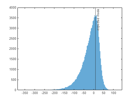

Compute PDF, CDF and inverse CDF with default methods

x=[10 25];
f=gx2pdf(x,w,k,l,s,m)

f =
    0.0121    0.0088

p=gx2cdf(x,w,k,l,s,m)

p =
    0.7150    0.8790

% find the median by using the inverse CDF function:
x_med=gx2inv(.5,w,k,l,s,m)

x_med =
-8.7657

% Compute quantiles for cdf values of 1e-3 and 1e-2, by supplying their log10 values:
x_q=gx2inv([-3 -2],w,k,l,s,m)

Warning: Imhof method output(s) too close to limit to compute exactly, so clipping. Check the flag output, and try stricter tolerances.

x_q =
 -218.3714 -149.2606

% verify that cdf values here are indeed 1e-3 and 1e-2
p=gx2cdf(x_q,w,k,l,s,m)

p =
    0.0010    0.0100

% Compute quantiles for complementary cdf values of 1e-3 and 1e-2, by supplying their log10 values:
x_q=gx2inv([-3 -2],w,k,l,s,m,'upper')

x_q =
   69.4899   51.0338

% verify that ccdf values here are indeed 1e-3 and 1e-2
p=gx2cdf(x_q,w,k,l,s,m,'upper')

p =
    0.0010    0.0100

% compute the PDF over most of the span of the distribution.
% with the 'full' argument, the span x is computed automatically.
[f,~,x]=gx2pdf('full',w,k,l,s,m);
 
% now compare the sampled histogram with the computed PDF
figure; hold on
plot(x,f)
histogram(r,'normalization','pdf','displaystyle','stairs')
xline(x_med,'-',{'median'},'labelorientation','aligned') % mark the computed median
xlim([-250 100])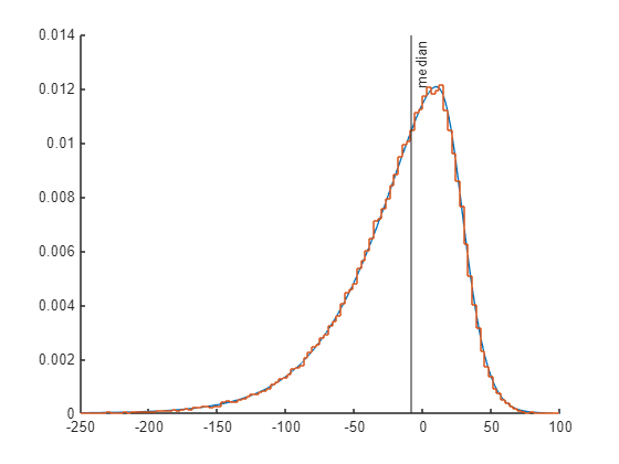

% compute CDF over most of the span of the distribution.
% the 'full' argument uses the IFFT method, good for quick rough plots,
% but less accurate (esp. for CDF) than some other methods
[p,~,x]=gx2cdf('full',w,k,l,s,m);
 
% now compare the sampled histogram with the computed CDF
figure; hold on
plot(x,p)
histogram(r,'normalization','cdf','displaystyle','stairs')
% mark the computed median, and verify that it sits at 0.5 on the vertical axis:
xline(x_med,'-',{'median'},'labelorientation','aligned')
yline(0.5)
xlim([-200 100])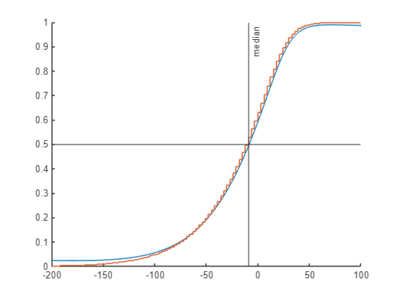

Compute CDF, PDF and inverse CDF with each exact method and its settings

A non-elliptic distribution

w=[-2 -5 2];
k=[2 1 3];
l=[0 4 4];
s=3;
m=-20;
 
% first find the quantile points at 0.1% in each tail
x_bounds=gx2inv([0.001 0.999],w,k,l,s,m)

x_bounds =
 -142.7703   24.8079

% now compute within this range
x=linspace(x_bounds(1),x_bounds(2),50);
 
% compute CDF
p_ifft=gx2cdf(x,w,k,l,s,m,'method','ifft');
p_imhof=gx2cdf(x,w,k,l,s,m,'method','imhof');
p_ray=gx2cdf(x,w,k,l,s,m,'method','ray','n_rays',1e4);
figure; hold on
plot(x,p_ifft,'-k')
plot(x,p_imhof,'.b')
plot(x,p_ray,'or')
legend('IFFT','Imhof','ray')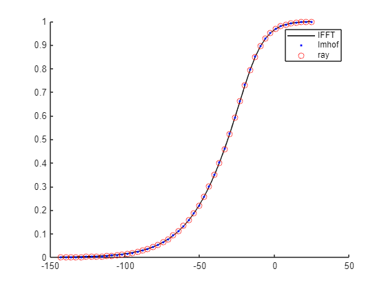

% compute PDF
f_ifft=gx2pdf(x,w,k,l,s,m,'method','ifft');
f_imhof=gx2pdf(x,w,k,l,s,m,'method','imhof');
f_ray=gx2pdf(x,w,k,l,s,m,'method','ray','n_rays',1e6);
 
figure; hold on
plot(x,f_ifft,'-k')
plot(x,f_imhof,'.b')
plot(x,f_ray,'or')
legend('IFFT','Imhof','ray')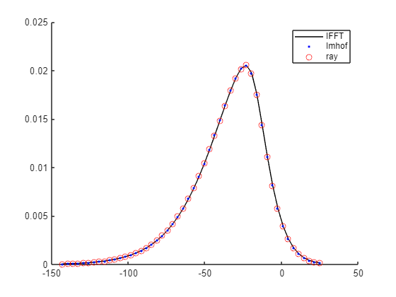

% Compute quantiles for tiny cdf values of 1e-1000 and 1e-2000, by supplying
% their log10 values. Use a forward cdf method that can get down to such tiny values.
% Here we use the infinite-tail approximation.
x_q=gx2inv([-1e3 -2e3],w,k,l,s,m,'method','tail')

Warning: Some output values are too small for double precision. Returning their log10 values, which are negative.

x_q =
10^4 ×
   -2.4365   -4.7950

% now verify using an exact cdf method that cdf values here are indeed 1e-1000 and 1e-2000:
p=gx2cdf(x_q,w,k,l,s,m,'method','ray','n_rays',1e7)

Warning: Some output values are too small for double precision. Returning their log10 values, which are negative.

p =
10^3 ×
   -1.0024   -2.0066

% now do the same for the upper tail:
x_q=gx2inv([-1e3 -2e3],w,k,l,s,m,'upper','method','tail')

Warning: Some output values are too small for double precision. Returning their log10 values, which are negative.

x_q =
10^4 ×
    0.9724    1.9159

p=gx2cdf(x_q,w,k,l,s,m,'upper','method','ray','n_rays',1e7)

Warning: Some output values are too small for double precision. Returning their log10 values, which are negative.

p =
10^3 ×
   -1.0021   -2.0048

An elliptic distribution

Here we can use Ruben's method too.

w=[3 4 5];
k=[1 2 3];
l=[2 3 7];
s=0;
m=-100;
 
% first find the quantile points at 0.1% in each tail
x_bounds=gx2inv([0.001 0.999],w,k,l,s,m)

x_bounds =
  -90.5258  122.3200

% now compute within this range
x=linspace(x_bounds(1),x_bounds(2),50);
 
% compute CDF
p_ifft=gx2cdf(x,w,k,l,s,m,'method','ifft');
p_imhof=gx2cdf(x,w,k,l,s,m,'method','imhof');
p_ray=gx2cdf(x,w,k,l,s,m,'method','ray','n_rays',1e4);
p_ruben=gx2cdf(x,w,k,l,s,m,'method','ruben');
 
figure; hold on
plot(x,p_ifft,'-k')
plot(x,p_imhof,'.b')
plot(x,p_ray,'or')
plot(x,p_ruben,'og','MarkerSize',8)
legend('IFFT','Imhof','ray', 'Ruben')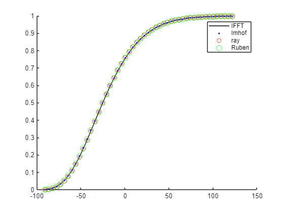

% compute PDF
f_ifft=gx2pdf(x,w,k,l,s,m,'method','ifft');
f_imhof=gx2pdf(x,w,k,l,s,m,'method','imhof');
f_ray=gx2pdf(x,w,k,l,s,m,'method','ray','n_rays',1e6);
f_ruben=gx2pdf(x,w,k,l,s,m,'method','ruben');
 
figure; hold on
plot(x,f_ifft,'-k')
plot(x,f_imhof,'.b')
plot(x,f_ray,'or')
plot(x,f_ruben,'og','MarkerSize',8)
legend('IFFT','Imhof','ray', 'Ruben')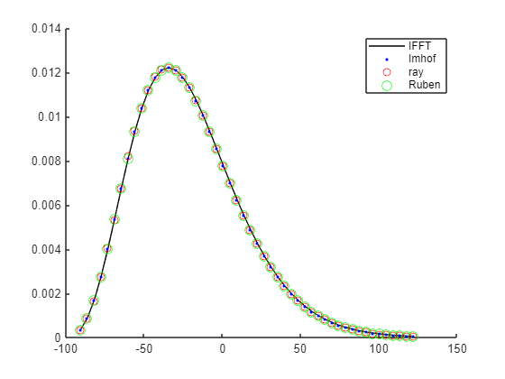

% Compute quantiles for tiny cdf values of 1e-1000 and 1e-2000, by supplying
% their log10 values. Use a forward cdf method that can get down to such tiny values.
% Here we use the ellipse approximation, with 'x_scale', 'log', which allows to specify
% log10 values of x measured from the finite tail m.
x_q=gx2inv([-1e3 -2e3],w,k,l,s,m,'method','ellipse','x_scale','log')

x_q =
 -331.2746 -664.6080

% this means that the computed quantiles are 1e-331 and 1e-664 above m
 
% now verify using the forward cdf method that cdf values here are indeed 1e-1000 and 1e-2000:
p=gx2cdf(x_q,w,k,l,s,m,'method','ellipse','x_scale','log')

p =
10^3 ×
   -1.0000   -2.0000

Compute CDF and PDF in the far tails, using some tail approximation methods too

Ray, tail and Imhof methods are best for infinite tails.

Compute CDF in an infinite lower tail

w=[1 2 -3 -4];
k=[6 5 4 3];
l=[5 10 0 0];
s=10;
m=-50;
 
x=linspace(-500,200,40);
 
p_ifft=gx2cdf(x,w,k,l,s,m,'method','ifft','span',1e7,'n_grid',1e7);
p_imhof=gx2cdf(x,w,k,l,s,m,'method','imhof','abstol',0,'reltol',1e-10);

Warning: Imhof method output(s) too close to limit to compute exactly, so clipping. Check the flag output, and try stricter tolerances.

p_ray=gx2cdf(x,w,k,l,s,m,'method','ray','n_rays',1e6);
p_pearson=gx2cdf(x,w,k,l,s,m,'method','pearson'); % pearson sucks
 
% tail approximation for lower tail. Mentioning 'lower' is needed here.
% For output values that are too small for double precision, it returns
% their log10 values, which are negative.
p_tail=gx2cdf(x,w,k,l,s,m,'lower','method','tail');
% convert all output values to their log10
p_tail(p_tail>0)=log10(p_tail(p_tail>0));
 
figure; hold on
plot(x,log10(p_ifft),'-k')
plot(x,log10(p_ray),'or')
plot(x,p_tail,'-g')
plot(x,log10(p_pearson),'.c','MarkerSize',15)
plot(x,log10(p_imhof),'.b')
 
axis([-5e2 200 -30 0])
 
legend('IFFT','ray','tail', 'pearson','Imhof')
ylabel('$\log_{10} p$','Interpreter','latex')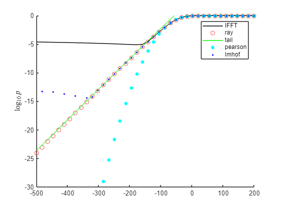

Compute PDF in an infinite upper tail

x=linspace(0,500,40);
 
f_ifft=gx2pdf(x,w,k,l,s,m,'method','ifft','span',1e7,'n_grid',1e7);
f_imhof=gx2pdf(x,w,k,l,s,m,'method','imhof','abstol',0,'reltol',1e-1);

Warning: Imhof method output(s) too close to limit to compute exactly, so clipping. Check the flag output, and try stricter tolerances.

f_ray=gx2pdf(x,w,k,l,s,m,'method','ray','n_rays',1e6);
f_pearson=gx2pdf(x,w,k,l,s,m,'method','pearson');
 
% tail approximation for upper tail. Mentioning 'upper' is needed here.
f_tail=gx2pdf(x,w,k,l,s,m,'upper','method','tail');
 
figure; hold on
plot(x,log10(f_ifft),'-k')
plot(x,log10(f_ray),'or')
plot(x,log10(f_tail),'-g')
plot(x,log10(f_pearson),'.c','MarkerSize',15)
plot(x,log10(f_imhof),'.b')
 
axis([0 500 -30 0])
 
legend('IFFT','ray','tail', 'pearson','Imhof')
ylabel('$\log_{10} f$','Interpreter','latex')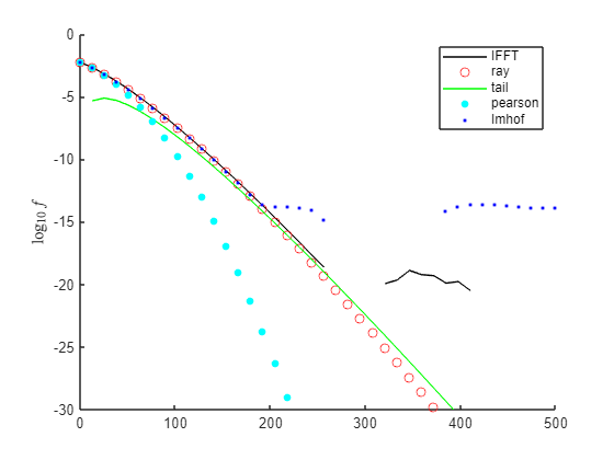

Compute CDF in a finite lower tail

Ruben and ellipse methods are best for finite tails.

w=[1 2 3 4];
k=[6 5 4 3];
l=[5 10 0 0];
s=0;
m=0;
 
x=logspace(-2,2,40);
 
p_ifft=gx2cdf(x,w,k,l,s,m,'method','ifft','span',1e7,'n_grid',1e7);
p_imhof=gx2cdf(x,w,k,l,s,m,'method','imhof','abstol',0,'reltol',1e-10);

Warning: Imhof method output(s) too close to limit to compute exactly, so clipping. Check the flag output, and try stricter tolerances.

p_ruben=gx2cdf(x,w,k,l,s,m,'method','ruben');
p_ray=gx2cdf(x,w,k,l,s,m,'method','ray','n_rays',1e5);
p_pearson=gx2cdf(x,w,k,l,s,m,'method','pearson');
p_ellipse=gx2cdf(x,w,k,l,s,m,'method','ellipse');
 
figure; hold on
plot(x,log10(p_ifft),'-k')
plot(x,log10(p_ray),'or','MarkerSize',8)
plot(x,log10(p_ellipse),'-g')
plot(x,log10(p_pearson),'.c','MarkerSize',15)
plot(x,log10(p_imhof),'.b')
plot(x,log10(p_ruben),'om','MarkerSize',4)
 
set(gca,'xscale','log')
legend('IFFT','ray','ellipse', 'pearson','Imhof','Ruben','Location', 'southeast')
ylabel('$\log_{10} p$','Interpreter','latex')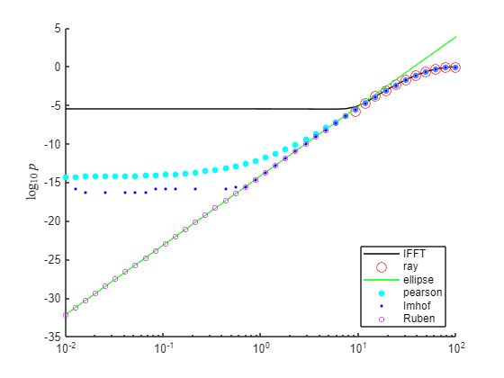

Distribution of quadratic form of a normal variable

Normal parameters:

mu=[5;6]; % mean
v=[2 1; 1 3]; % covariance matrix

Sample normal random vectors:

x=mvnrnd(mu,v,1e5)';
figure; plot(x(1,:),x(2,:),'.')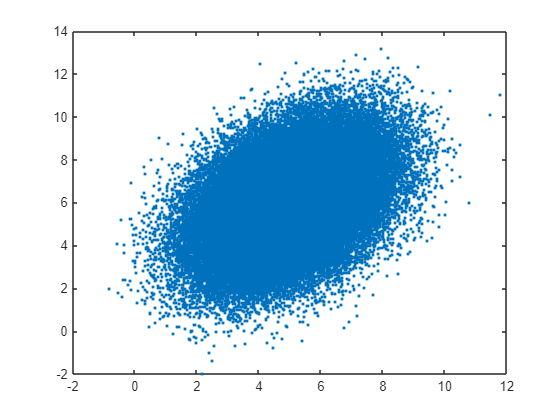

Quadratic form $q(\mathbf{x})=(x_1+x_2)^2-x_1-1$ = [x1;x2]'*[1 1; 1 1]*[x1;x2] + [-1;0]'*[x1;x2] -1

quad.q2=[1 1; 1 1];
quad.q1=[-1;0];
quad.q0=-1;

Compute the quadratic form q for the sample of normal vectors:

q=dot(x,quad.q2*x)+quad.q1'*x+quad.q0;

Get generalized chi-square parameters corresponding to this quadratic form:

[w,k,l,s,m]=norm_quad_to_gx2_params(mu,v,quad)

w =
7.0000

k =
1

lambda =
16.6188

s =
0.8452

m =
-1.3316

Compare the sampled and calculated distributions of q:

[f,~,x]=gx2pdf('full',w,k,l,s,m);
plot(x,f); hold on
histogram(q,'normalization','pdf','displaystyle','stairs')
xlim([0 400])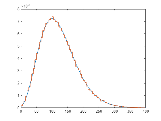

Compare the sampled and calculated means and variances:

[mu_q,v_q]=gx2stat(w,k,l,s,m);
[mu_q mean(q)]

ans =
  122.0000  122.1560

[v_q var(q)]

ans =
10^3 ×
    3.3560    3.3730

Compare the sampled and calculated probabilities $p(q(\mathbf{x})<50)$:

mean(q<50)

ans =
0.0859

gx2cdf(50,w,k,l,s,m)

ans =
0.0856

Find a canonical quadratic form of a standard multinormal corresponding to these generalized chi-square parameters:

quad=gx2_to_norm_quad_params(w,k,l,s,m)

quad =
struct with fields:
    q2: [2×2 double]
    q1: [2×1 double]
    q0: 115

Compute characteristic function

t=linspace(-1,1,1e3);
phi=gx2char(t,w,k,l,s,m);
figure; plot(phi,'-o')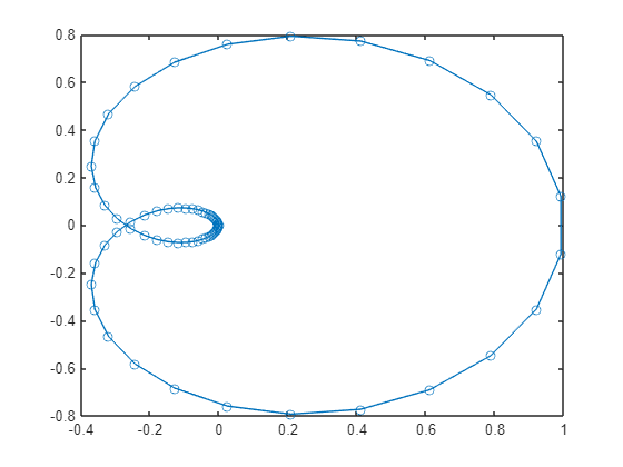

1st & 2nd derivatives (gradient & Hessian) of CDF wrt distribution parameters

This uses first and second derivatives computed analytically (faster and more accurate), than finite-differencing the cdf, which is slower and noisier.

Gradient and Hessian wrt the 'native' parameters

Take a generalized chi-square and a point $x_0$, and ask how the cdf $F(x_0)$ changes as we nudge the distribution parameters.

w=[1 -5 2];
k=[1 2 3];
l=[2 3 7];
s=2;
m=5;
x0=10;
 
% The gradient is a flat vector over all parameters, in the canonical order
% [w, k, l, s, m] (all of w, then all of k, ...); the Hessian is the
% matching square matrix.
[grad,hess]=cdf_grad_gx2(x0,w,k,l,s,m)

grad =
   -0.0593
   -0.0647
   -0.1834
   -0.0204
    0.0934
   -0.0402
   -0.0202
    0.0803
   -0.0389
    0.0000

hess =
    0.0072   -0.0058    0.0131   -0.0192    0.0010    0.0021   -0.0185    0.0041    0.0024    0.0004    0.0008
   -0.0058   -0.0168   -0.0132   -0.0023   -0.0035   -0.0043   -0.0022    0.0007   -0.0036    0.0002   -0.0025
    0.0131   -0.0132    0.0602    0.0039   -0.0048   -0.0113    0.0041    0.0057   -0.0091    0.0008    0.0036
   -0.0192   -0.0023    0.0039    0.0002    0.0011    0.0005    0.0002    0.0020    0.0006    0.0002    0.0001
    0.0010   -0.0035   -0.0048    0.0011   -0.0120    0.0016    0.0008   -0.0133    0.0004   -0.0007    0.0015
    0.0021   -0.0043   -0.0113    0.0005    0.0016    0.0011    0.0006    0.0034    0.0014    0.0003    0.0003
   -0.0185   -0.0022    0.0041    0.0002    0.0008    0.0006    0.0003    0.0017    0.0007    0.0002    0.0002
    0.0041    0.0007    0.0057    0.0020   -0.0133    0.0034    0.0017   -0.0130    0.0024   -0.0005    0.0022
    0.0024   -0.0036   -0.0091    0.0006    0.0004    0.0014    0.0007    0.0024    0.0016    0.0002    0.0005
    0.0004    0.0002    0.0008    0.0002   -0.0007    0.0003    0.0002   -0.0005    0.0002    0.0000    0.0002

Taylor picture: vary one native parameter and predict the cdf

We compute derivatives only wrt λ, then use the first and second derivative of $\lambda_1$ to build the second-order Taylor model of $F(x_0)$ as $\lambda_1$ moves.

$F(x_0),$ $\frac{\partial F(x_0)}{\partial \lambda_1}$ and $\frac{\partial^2 F(x_0)}{\partial \lambda_1^2}$:

F0=gx2cdf(x0,w,k,l,s,m);
[g,H]=cdf_grad_gx2(x0,w,k,l,s,m,'wrt',{'l'});
gl=g(1); Hl=H(1,1);                     
 
delta=linspace(-50,50,100);
Ftrue=arrayfun(@(d) gx2cdf(x0,w,k,l+[d 0 0],s,m),delta);

Warning: Imhof method output(s) too close to limit to compute exactly, so clipping. Check the flag output, and try stricter tolerances.

Ftaylor=F0+gl*delta+0.5*Hl*delta.^2;
 
figure; hold on
plot(l(1)+delta,Ftrue,'k-');
plot(l(1)+delta,Ftaylor,'-b');
plot(l(1),F0,'bo','MarkerFaceColor','b');
xlabel('\lambda_1'); ylabel('F(x_0)');
axis([-50 50 0 1])
legend('true cdf','2nd-order Taylor','location','best');
legend boxoff
title('cdf sensitivity to a non-centrality \lambda_1');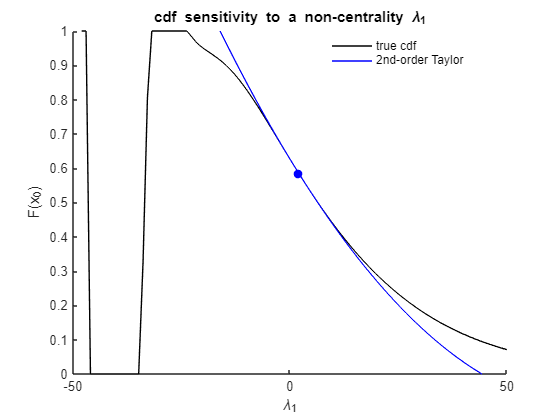

Gradient and Hessian wrt the parameters of the quadratic boundary

mu=[1;2]; v=[2 1; 1 3];
quad.q2=[1 1; 1 1]; quad.q1=[-1;0]; quad.q0=-1;
x0=0;
 
[grad,hess]=cdf_grad_norm_quad(x0,mu,v,quad);
disp('dF/dQ2:'); disp(grad.q2);

dF/dQ2:
   -0.0628    0.0289
    0.0289   -0.0784

disp('dF/dq1:'); disp(grad.q1);

dF/dq1:
    0.0128
   -0.0588

fprintf('dF/dq0: %.4f\n',grad.q0);

dF/dq0: -0.0962

Taylor picture: vary one boundary parameter and predict the cdf

We compute the second-order Taylor approximation of $F(x_0)$ wrt variations in $\mathbf{Q}_{11}$.

$F(x_0),$ $\frac{\partial F(x_0)}{\partial \mathbf{Q}{11}}$ and $\frac{\partial^2 F(x_0)}{\partial \mathbf{Q}{11}^2}$:

[w2,k2,l2,s2,m2]=norm_quad_to_gx2_params(mu,v,quad);
 
F0=gx2cdf(x0,w2,k2,l2,s2,m2);
g11=grad.q2(1,1); H11=hess.q2q2(1,1,1,1);
 
delta=linspace(-2,2,100);
Ftrue=arrayfun(@(d) probq(mu,v,quad,d,x0),delta);
Ftaylor=F0+g11*delta+0.5*H11*delta.^2;
 
figure; hold on 
plot(quad.q2(1,1)+delta,Ftrue,'k-');
plot(quad.q2(1,1)+delta,Ftaylor,'-b');
plot(quad.q2(1,1),F0,'bo','MarkerFaceColor','b');
xlabel('Q_2(1,1)'); ylabel('F(x_0)');
legend('true cdf','2nd-order Taylor','location','best');
legend boxoff
title('cdf sensitivity to boundary coeff. Q_2(1,1)');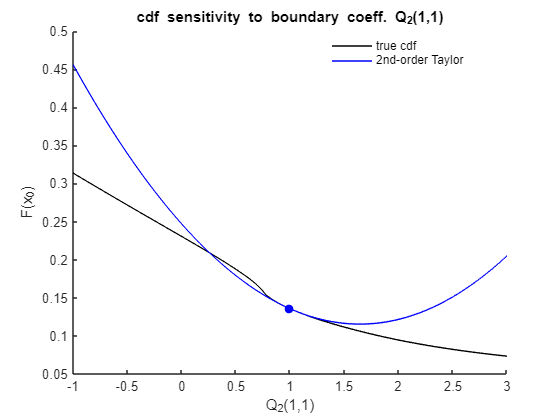

%% helper: probability with the Q2(1,1) coefficient perturbed by d
function p=probq(mu,v,quad,d,x0)
    quad.q2(1,1)=quad.q2(1,1)+d;
    [w,k,l,s,m]=norm_quad_to_gx2_params(mu,v,quad);
    p=gx2cdf(x0,w,k,l,s,m);
end

More classification-related functionality

Additional functionality related to binary Gaussian classification models, that you may find in the corresponding gx2-py python package (such as computing the optimal classification boundary between two Gaussians, and the gradient and Hessian of the classification error with respect to it), are in the Matlab toolbox 'Integrate and Classify Normal Distributions', specialized for Gaussian classification applications.